Lebesgue integration

In mathematics, Lebesgue integration, named after French mathematician Henri Lebesgue (1875-1941), refers to both the general theory of integration of a function with respect to a general measure, and to the specific case of integration of a function defined on a subset of the real line or a higher dimensional Euclidean space with respect to the Lebesgue measure. This article focuses on the more general concept.

Lebesgue integration plays an important role in real analysis, the axiomatic theory of probability, and many other fields in the mathematical sciences.

The integral of a non-negative function can be regarded in the simplest case as the area between the graph of that function and the x-axis. The Lebesgue integral is a construction that extends the integral to a larger class of functions defined over spaces more general than the real line.

For non-negative functions with a smooth enough graph (such as continuous functions on closed bounded intervals), the area under the curve is defined as the integral and computed using techniques of approximation of the region by polygons (see Simpson's rule). For more irregular functions (such as the limiting processes of mathematical analysis and probability theory), better approximation techniques are required in order to define a suitable integral.

1 Introduction
2 Construction of the Lebesgue integral
3 Limitations of the Riemann integral
4 Basic theorems of the Lebesgue integral
5 Proof techniques
6 Alternative formulations
7 See also
8 Notes
9 References

Introduction

The integral of a function f between limits a and b can be interpreted as the area under the graph of f. This is easy to understand for familiar functions such as polynomials, but what does it mean for more exotic functions? In general, what is the class of functions for which "area under the curve" makes sense? The answer to this question has great theoretical and practical importance.

As part of a general movement toward rigour in mathematics in the nineteenth century, attempts were made to put the integral calculus on a firm foundation. The Riemann integral, proposed by Bernhard Riemann (1826–1866), is a broadly successful attempt to provide such a foundation. Riemann's definition starts with the construction of a sequence of easily-calculated areas which converge to the integral of a given function. This definition is successful in the sense that it gives the expected answer for many already-solved problems, and gives useful results for many other problems.

However, Riemann integration does not interact well with taking limits of sequences of functions, making such limiting processes difficult to analyze. This is of prime importance, for instance, in the study of Fourier series, Fourier transforms and other topics. The Lebesgue integral is better able to describe how and when it is possible to take limits under the integral sign. The Lebesgue definition considers a different class of easily-calculated areas than the Riemann definition, which is the main reason the Lebesgue integral is better behaved. The Lebesgue definition also makes it possible to calculate integrals for a broader class of functions. For example, the Dirichlet function, which is 0 where its argument is irrational and 1 otherwise, has a Lebesgue integral, but it does not have a Riemann integral.

Construction of the Lebesgue integral

The discussion that follows parallels the most common expository approach to the Lebesgue integral. In this approach, the theory of integration has two distinct parts:

A theory of measurable sets and measures on these sets.
A theory of measurable functions and integrals on these functions.

Measure theory

Further information: Measure (mathematics)

Measure theory was initially created to provide a useful abstraction of the notion of length of subsets of the real line and, more generally, area and volume of subsets of Euclidean spaces. In particular, it provided a systematic answer to the question of which subsets of R have a length. As was shown by later developments in set theory (see non-measurable set), it is actually impossible to assign a length to all subsets of R in a way which preserves some natural additivity and translation invariance properties. This suggests that picking out a suitable class of measurable subsets is an essential prerequisite.

The Riemann integral uses the notion of length explicitly. Indeed, the element of calculation for the Riemann integral is the rectangle [a, b] × [c, d], whose area is calculated to be (b − a)(d − c). The quantity b − a is the length of the base of the rectangle and d − c is the height of the rectangle. Riemann could only use planar rectangles to approximate the area under the curve because there was no adequate theory for measuring more general sets.

In the development of the theory in most modern textbooks (after 1950), the approach to measure and integration is axiomatic. This means that a measure is any function μ defined on a certain class X of subsets of a set E, which satisfies a certain list of properties. These properties can be shown to hold in many different cases.

Integration

We start with a measure space (E, X, μ) where E is a set, X is a σ-algebra of subsets of E and μ is a (non-negative) measure on E, defined on the sets of X.

For example, E can be Euclidean n-space Rⁿ or some Lebesgue measurable subset of it, X will be the σ-algebra of all Lebesgue measurable subsets of E, and μ will be the Lebesgue measure. In the mathematical theory of probability, we confine our study to a probability measure μ, which satisfies $\mu(E) = 1$ .

In Lebesgue's theory, integrals are defined for a class of functions called measurable functions. A function ƒ is measurable if the pre-image of every closed interval is in X:

$f^{-1}([a,b]) \in X \text{ for all }a<b.$

It can be shown that this is equivalent to requiring that the pre-image of any Borel subset of R be in X. We will make this assumption henceforth. The set of measurable functions is closed under algebraic operations, but more importantly the class is closed under various kinds of pointwise sequential limits:

$\sup_{k \in \mathbb{N}} f_k, \quad \liminf_{k \in \mathbb{N}} f_k, \quad \limsup_{k \in \mathbb{N}} f_k$

are measurable if the original sequence (ƒ_k)_k, where k ∈ N, consists of measurable functions.

We build up an integral

$\int_E f \, d \mu = \int_E f\left(x\right)\, \mu\left(dx\right)$

for measurable real-valued functions ƒ defined on E in stages:

Indicator functions: To assign a value to the integral of the indicator function $1_S$ of a measurable set S consistent with the given measure μ, the only reasonable choice is to set:

$\int 1_S \, \mathrm{d} \mu = \mu (S).$

Notice that the result may be equal to +∞, unless μ is a finite measure.

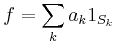
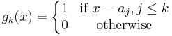
Simple functions: A finite linear combination of indicator functions

$\sum_k a_k 1_{S_k}$

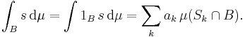
where the coefficients a_k are real numbers and the sets S_k are measurable, is called a measurable simple function. We extend the integral by linearity to non-negative measurable simple functions. When the coefficients a_k are non-negative, we set

$\int \bigg(\sum_k a_k 1_{S_k}\bigg) \, \mathrm{d} \mu = \sum_k a_k \int 1_{S_k} \, \mathrm{d} \mu = \sum_k a_k \, \mu(S_k).$

The convention 0 × ∞ = 0 must be used, and the result may be infinite. Even if a simple function can be written in many ways as a linear combination of indicator functions, the integral will always be the same; this can be shown using the additivity property of measures.

Some care is needed when defining the integral of a real-valued simple function, in order to avoid the undefined expression ∞ − ∞: one assumes that the representation

$f = \sum_k a_k 1_{S_k}$

is such that μ(S_k) < ∞ whenever a_k ≠ 0. Then the above formula for the integral of ƒ makes sense, and the result does not depend upon the particular representation of ƒ satisfying the assumptions.

If B is a measurable subset of E and s a measurable simple function one defines

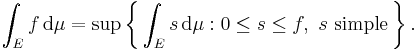
$\int_B s \, \mathrm{d}\mu = \int 1_B \, s \, \mathrm{d}\mu = \sum_k a_k \, \mu(S_k \cap B).$

Non-negative functions: Let ƒ be a non-negative measurable function on E which we allow to attain the value +∞, in other words, ƒ takes non-negative values in the extended real number line. We define

$\int_E f \, \mathrm{d}\mu = \sup\left\{\,\int_E s\, \mathrm{d}\mu�: 0 \le s \le f,\ s\ \text{simple}\,\right\}.$

We need to show this integral coincides with the preceding one, defined on the set of simple functions. When E is a segment [a, b], there is also the question of whether this corresponds in any way to a Riemann notion of integration. It is possible to prove that the answer to both questions is yes.

We have defined the integral of ƒ for any non-negative extended real-valued measurable function on E. For some functions, this integral ∫_E ƒ dμ will be infinite.

Signed functions: To handle signed functions, we need a few more definitions. If ƒ is a measurable function of the set E to the reals (including ± ∞), then we can write

$f = f^%2B - f^-, \quad$

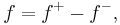
where

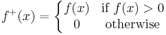
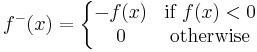
$f^%2B(x) = \left\{\begin{matrix} f(x) & \text{if } f(x) > 0 \\ 0 & \text{otherwise} \end{matrix}\right.$

$f^-(x) = \left\{\begin{matrix} -f(x) & \text{if } f(x) < 0 \\ 0 & \text{otherwise} \end{matrix}\right.$

Note that both ƒ⁺ and ƒ⁻ are non-negative measurable functions. Also note that

$|f| = f^%2B %2B f^-. \quad$

We say that the Lebesgue integral of the measurable function $f$ exists, or is defined if at least one of $\int f^%2B \, d\mu$ and $\int f^- \, d\mu$ is finite:

$\min(\int f^%2B \, d \mu, \int f^- \, d \mu) < \infty.$

In this case we define

$\int f \, d \mu = \int f^%2B \, d \mu - \int f^- \, d \mu.$

$\int |f| \, d \mu < \infty,$

we say that ƒ is Lebesgue integrable.

It turns out that this definition gives the desirable properties of the integral.

Complex valued functions can be similarly integrated, by considering the real part and the imaginary part separately.

Intuitive interpretation

To get some intuition about the different approaches to integration, let us imagine that it is desired to find a mountain's volume (above sea level).

The Riemann-Darboux approach: Divide the base of the mountain into a grid of 1 meter squares. Measure the altitude of the mountain at the center of each square. The volume on a single grid square is approximately 1x1x(altitude), so the total volume is the sum of the altitudes.

The Lebesgue approach: Draw a contour map of the mountain, where each contour is 1 meter of altitude apart. The volume of earth contained in a single contour is approximately that contour's area times its height. So the total volume is the sum of these volumes.

Folland^[1] summarizes the difference between the Riemann and Lebesgue approaches thus: "to compute the Riemann integral of f, one partitions the domain [a, b] into subintervals", while in the Lebesgue integral, "one is in effect partitioning the range of f".

Example

Consider the indicator function of the rational numbers, 1_Q. This function is nowhere continuous.

$1_{\mathbb Q}$ is not Riemann-integrable on [0,1]: No matter how the set [0,1] is partitioned into subintervals, each partition will contain at least one rational and at least one irrational number, since rationals and irrationals are both dense in the reals. Thus the upper Darboux sums will all be one, and the lower Darboux sums will all be zero.

$1_{\mathbb Q}$ is Lebesgue-integrable on [0,1] using the Lebesgue measure: Indeed it is the indicator function of the rationals so by definition

$\int_{[0,1]} 1_{\mathbb Q} \, d \mu = \mu(\mathbb Q \cap [0,1]) = 0,$

since $\mathbb Q$ is countable.

Domain of integration

A technical issue in Lebesgue integration is that the domain of integration is defined as a set (a subset of a measure space), with no notion of orientation. In elementary calculus, one defines integration with respect to an orientation: $\textstyle{\int_b^a f�:= - \int_a^b f}.$ Generalizing this to higher dimensions yields integration of differential forms. By contrast, Lebesgue integration provides an alternative generalization, integrating over subsets with respect to a measure; this can be notated as $\int_A f\,d\mu = \int_{[a,b]} f\,d\mu$ to indicate integration over a subset A. For details on the relation between these generalizations, see Differential form: Relation with measures.

Limitations of the Riemann integral

Here we discuss the limitations of the Riemann integral and the greater scope offered by the Lebesgue integral. We presume a working understanding of the Riemann integral.

With the advent of Fourier series, many analytical problems involving integrals came up whose satisfactory solution required interchanging limit processes and integral signs. However, the conditions under which the integrals

$\sum_k \int f_k(x) dx$ and $\int \bigg[\sum_k f_k(x) \bigg] dx$

are equal proved quite elusive in the Riemann framework. There are some other technical difficulties with the Riemann integral. These are linked with the limit-taking difficulty discussed above.

Failure of monotone convergence. As shown above, the indicator function 1_Q on the rationals is not Riemann integrable. In particular, the Monotone convergence theorem fails. To see why, let {a_k} be an enumeration of all the rational numbers in [0,1] (they are countable so this can be done.) Then let

$g_k(x) = \left\{\begin{matrix} 1 & \mbox{if } x = a_j, j\leq k \\ 0 & \mbox{otherwise} \end{matrix} \right.$

The function g_k is zero everywhere except on a finite set of points, hence its Riemann integral is zero. The sequence g_k is also clearly non-negative and monotonically increasing to 1_Q, which is not Riemann integrable.

Unsuitability for unbounded intervals. The Riemann integral can only integrate functions on a bounded interval. It can however be extended to unbounded intervals by taking limits, so long as this doesn't yield an answer such as $\infty -\infty$ .

Integrating on structures other than Euclidean space. The Riemann integral is inextricably linked to the order structure of the line.

Basic theorems of the Lebesgue integral

The Lebesgue integral does not distinguish between functions which differ only on a set of μ-measure zero. To make this precise, functions f and g are said to be equal almost everywhere (a.e.) if

$\mu(\{x \in E: f(x) \neq g(x)\}) = 0.$

If f, g are non-negative measurable functions (possibly assuming the value +∞) such that f = g almost everywhere, then

$\int f \, \mathrm{d} \mu = \int g \, \mathrm{d} \mu.$

To wit, the integral respects the equivalence relation of almost-everywhere equality.

If f, g are functions such that f = g almost everywhere, then f is Lebesgue integrable if and only if g is Lebesgue integrable and the integrals of f and g are the same.

The Lebesgue integral has the following properties:

Linearity: If f and g are Lebesgue integrable functions and a and b are real numbers, then af + bg is Lebesgue integrable and

$\int (a f %2B bg) \, \mathrm{d} \mu = a \int f \, \mathrm{d}\mu %2B b \int g \, \mathrm{d}\mu.$

Monotonicity: If f ≤ g, then

$\int f \, \mathrm{d} \mu \leq \int g \, \mathrm{d} \mu.$

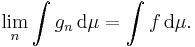
Monotone convergence theorem: Suppose {f_k}_k ∈ N is a sequence of non-negative measurable functions such that

$f_k(x) \leq f_{k%2B1}(x) \quad \forall k\in \mathbb{N}, \, \forall x \in E.$

Then

$\lim_k \int f_k \, \mathrm{d} \mu = \int \lim_k f_k \, \mathrm{d} \mu.$

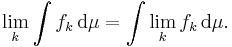
Note: The value of any of the integrals is allowed to be infinite.

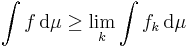
Fatou's lemma: If {f_k}_k ∈ N is a sequence of non-negative measurable functions, then

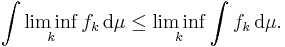
$\int \liminf_k f_k \, \mathrm{d} \mu \leq \liminf_k \int f_k \, \mathrm{d} \mu.$

Again, the value of any of the integrals may be infinite.

Dominated convergence theorem: If {f_k}_k ∈ N is a sequence of complex measurable functions with pointwise limit f, and if there is a Lebesgue integrable function g (i.e., g belongs to the space L¹) such that |f_k| ≤ g for all k, then f is Lebesgue integrable and

$\lim_k \int f_k \, \mathrm{d} \mu = \int f \, \mathrm{d} \mu.$

Proof techniques

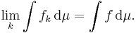
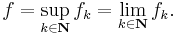
To illustrate some of the proof techniques used in Lebesgue integration theory, we sketch a proof of the above mentioned Lebesgue monotone convergence theorem. Let {f_k}_k ∈ N be a non-decreasing sequence of non-negative measurable functions and put

$f = \sup_{k \in \mathbf{N}} f_k = \lim_{k \in \mathbf{N}} f_k.$

By the monotonicity property of the integral, it is immediate that:

$\int f \, \mathrm{d} \mu \geq \lim_k \int f_k \, \mathrm{d} \mu$

and the limit on the right exists, since the sequence is monotonic. We now prove the inequality in the other direction. It follows from the definition of integral that there is a non-decreasing sequence (g_n) of non-negative simple functions such that g_n ≤ f and

$\lim_n \int g_n \, \mathrm{d} \mu = \int f \, \mathrm{d} \mu.$

Therefore, it suffices to prove that for each n ∈ N,

$\int g_n \, \mathrm{d} \mu \leq \lim_k \int f_k \, \mathrm{d} \mu.$

We will show that if g is a simple function and

$\lim_k f_k(x) \geq g(x)$

almost everywhere, then

$\lim_k \int f_k \, \mathrm{d} \mu \geq \int g \, \mathrm{d} \mu.$

By breaking up the function g into its constant value parts, this reduces to the case in which g is the indicator function of a set. The result we have to prove is then

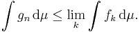
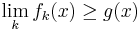
Suppose A is a measurable set and {f_k}_k ∈ N is a nondecreasing sequence of non-negative measurable functions on E such that

$\lim_k f_k (x) \geq 1$

for almost all x ∈ A. Then

$\lim_k \int f_k \, \mathrm{d}\mu \geq \mu(A).$

To prove this result, fix ε > 0 and define the sequence of measurable sets

$B_k = \{x \in A: f_k(x) \geq 1 - \epsilon \}.$

By monotonicity of the integral, it follows that for any k ∈ N,

$(1 - \epsilon) \mu(B_k) = \int (1 - \epsilon) 1_{B_k} \, \mathrm{d} \mu \leq \int f_k \, \mathrm{d} \mu$

Because almost every x will be in B_k for large enough k, we have

$\bigcup_k B_k = A,$

up to a set of measure 0. Thus by countable additivity of μ, and since B_k increases with k,

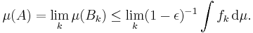
$\mu(A) = \lim_k \mu(B_k) \leq \lim_k (1 - \epsilon)^{-1} \int f_k \, \mathrm{d} \mu.$

As this is true for any positive ε the result follows.

Alternative formulations

It is possible to develop the integral with respect to the Lebesgue measure without relying on the full machinery of measure theory. One such approach is provided by Daniell integral.

There is also an alternative approach to developing the theory of integration via methods of functional analysis. The Riemann integral exists for any continuous function f of compact support defined on Rⁿ (or a fixed open subset). Integrals of more general functions can be built starting from these integrals. Let C_c be the space of all real-valued compactly supported continuous functions of R. Define a norm on C_c by

$\|f\| = \int |f(x)| dx.$

Then C_c is a normed vector space (and in particular, it is a metric space.) All metric spaces have Hausdorff completions, so let L¹ be its completion. This space is isomorphic to the space of Lebesgue integrable functions modulo the subspace of functions with integral zero. Furthermore, the Riemann integral ∫ is a uniformly continuous functional with respect to the norm on C_c, which is dense in L¹. Hence ∫ has a unique extension to all of L¹. This integral is precisely the Lebesgue integral.

This approach can be generalised to build the theory of integration with respect to Radon measures on locally compact spaces. It is the approach adopted by Bourbaki (2004); for more details see Radon measures on locally compact spaces.

Notes

^ Gerald B. Folland, Real Analysis: Modern Techniques and Their Applications, 1984, p. 56.

References

Bartle, Robert G. (1995). The elements of integration and Lebesgue measure. Wiley Classics Library. New York: John Wiley & Sons Inc.. xii+179. ISBN 0-471-04222-6. | mr = 1312157

Bourbaki, Nicolas (2004). Integration. I. Chapters 1–6. Translated from the 1959, 1965 and 1967 French originals by Sterling K. Berberian. Elements of Mathematics (Berlin). Berlin: Springer-Verlag. xvi+472. ISBN 3-540-41129-1. | mr = 2018901

Dudley, Richard M. (1989). Real analysis and probability. The Wadsworth & Brooks/Cole Mathematics Series. Pacific Grove, CA: Wadsworth & Brooks/Cole Advanced Books & Software. xii+436. ISBN 0-534-10050-3. | mr = 982264 Very thorough treatment, particularly for probabilists with good notes and historical references.

Folland, Gerald B. (1999). Real analysis: Modern techniques and their applications. Pure and Applied Mathematics (New York) (Second ed.). New York: John Wiley & Sons Inc.. xvi+386. ISBN 0-471-31716-0. | mr = 1681462

Halmos, Paul R. (1950). Measure Theory. New York, N. Y.: D. Van Nostrand Company, Inc.. pp. xi+304. | mr = 0033869 A classic, though somewhat dated presentation.

Lebesgue, Henri (1904). Leçons sur l'intégration et la recherche des fonctions primitives. Paris: Gauthier-Villars

Lebesgue, Henri (1972) (in French). Oeuvres scientifiques (en cinq volumes). Geneva: Institut de Mathématiques de l'Université de Genève. pp. 405. | mr = 0389523

Loomis, Lynn H. (1953). An introduction to abstract harmonic analysis. Toronto-New York-London: D. Van Nostrand Company, Inc.. pp. x+190. | mr = 0054173 Includes a presentation of the Daniell integral.

Munroe, M. E. (1953). Introduction to measure and integration. Cambridge, Mass.: Addison-Wesley Publishing Company Inc.. pp. x+310. | mr = 0053186 Good treatment of the theory of outer measures.

Royden, H. L. (1988). Real analysis (Third ed.). New York: Macmillan Publishing Company. pp. xx+444. ISBN 0-02-404151-3. | mr = 1013117

Rudin, Walter (1976). Principles of mathematical analysis. International Series in Pure and Applied Mathematics (Third ed.). New York: McGraw-Hill Book Co.. pp. x+342. | mr = 0385023 Known as Little Rudin, contains the basics of the Lebesgue theory, but does not treat material such as Fubini's theorem.

Rudin, Walter (1966). Real and complex analysis. New York: McGraw-Hill Book Co.. pp. xi+412. | mr = 0210528 Known as Big Rudin. A complete and careful presentation of the theory. Good presentation of the Riesz extension theorems. However, there is a minor flaw (in the first edition) in the proof of one of the extension theorems, the discovery of which constitutes exercise 21 of Chapter 2.
Saks, Stanisław (1937). Theory of the Integral. Monografie Matematyczne. 7 (2nd ed.). Warszawa-Lwów: G.E. Stechert & Co.. pp. VI+347. JFM 63.0183.05. Zbl 0017.30004. http://matwbn.icm.edu.pl/kstresc.php?tom=7&wyd=10&jez=pl . English translation by Laurence Chisholm Young, with two additional notes by Stefan Banach.

Shilov, G. E.; Gurevich, B. L. (1977). Integral, measure and derivative: a unified approach. Translated from the Russian and edited by Richard A. Silverman. Dover Books on Advanced Mathematics. New York: Dover Publications Inc.. xiv+233. ISBN 0-486-63519-8. | mr = 0466463 Emphasizes the Daniell integral.

Integrals

Methods	Riemann integral · Lebesgue integral · Burkill integral · Bochner integral · Daniell integral · Darboux integral · Henstock–Kurzweil integral · Haar integral · Hellinger integral · Kolmogorov integral · Lebesgue–Stieltjes integral · Pettis integral · Pfeffer integral · Riemann–Stieltjes integral · Regulated integral

Improper Integrals	Improper integral · Gaussian integral

Stochastic integrals	Itō integral · Stratonovich integral · Skorokhod integral